
Lesson Nine
Chance - The Luck of the Draw
After successfully completing this lesson, you should be able to:
1. Describe the relationship between sample size and confidence
2. Interpret confidence interval and margin of error
3. Describe the relationship between sample size, margin of error and confidence interval
4. Make a decision as a health professional with confidence interval
5. Interpret the P-value
A street entertainer offers to give you $20 if you can guess the percentage of poker chips in his hat that are red. You can draw three chips from the hat without looking. One of three comes up red. What will you guess? 33%, right?
He offers to let you draw another 3 chips to improve your guess, but now you can only win $10. Will you guess 33% or pick another 3 chips? He says, to make it easier, you could pick 9 more chips, but now you can only win $5. What will you do?
This is similar to the dilemma we face in research. The more subjects we include in our study, the more confident we can be in our results. However, it costs more to include more subjects, so the net benefit of the research may be diminished. The comic below is certainly exaggerated, but it made a good point.
At what point does the increased cost outweigh the value of the additional information? How much uncertainty remains, when we finally select our subjects and collect our data? These are the essential questions of the source of error we call CHANCE.
One way to understand CHANCE is to use a sampling analogy. Assume you have a large group of people, which we call a population. Assume that 30% of these people are HIV+. You then randomly draw a sample of 20 people from this population. You would expect that 6 people in this group would be HIV+. But if you found 7, would you be shocked? No. You know that just by the "luck of the draw" (CHANCE), you're not going to get exactly 30% in every sample.
If you draw many samples of 20, you know that more samples will have 6 HIV+ people than any other number, though many will have 5 or 7 HIV+ people Some smaller number will have 4 or 8 HIV+ people. You would expect very few samples to have, say, 0 or 15 HIV+ people. What is being described here is a sampling distribution of a proportion. Similarly, with other statistics like average, average calculated from a sample may be different from the true average of the population from which the sample is drawn, just by the 'Luck of the draw" (CHANCE), as indicated below.
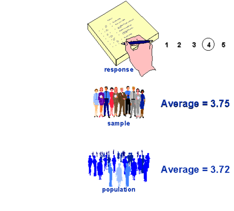
If we draw many samples and calculate an average from each sample, we will have a distribution of these averages - i.e. sampling distribution of the average.
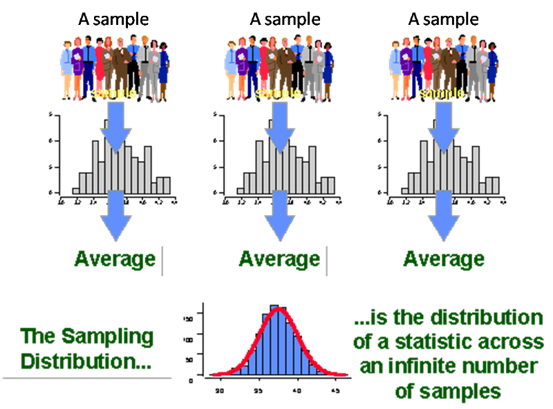
Though you do not need to understand exactly how, the sampling distribution is used to quantify the uncertainty created by "the luck of the draw." We quantify this uncertainty in two ways: confidence intervals and p-values.
Even if you aren't familiar with confidence intervals, you've probably unknowingly run across them. You've probably heard the term "Margin of Error" used along with the results of a survey of, say, a presidential poll.
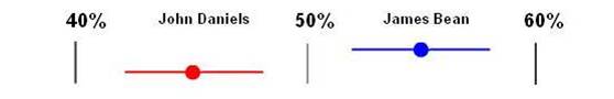
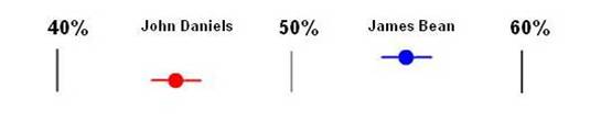
 After polling 1000 eligible voters, the Star-Tribune Newspaper reported that 55% of Americans would vote for James Bean and 45% for John F Daniels +/- 3%.
That plus or minus disclaimer is the margin of error. In other words, the margin of error means that James Bean could be favored by as much as 58 to 42 percent (55 + 3) or as low as 52 to 48 percent (55 - 3)-- a six percentage point spread (58-52 = 6). This spread is the Confidence Interval [1] (move your mouse over the colored text to find out more).
There's our friend the Margin of Error. It can be used whenever samples are taken and an estimate is made about a larger population. Did you also notice that the margin of error is half the confidence interval? So an easy way to know the confidence interval if all you know is the margin of error is to multiply the margin of error times two.
So remember the confidence interval = 2 times the Margin of Error
There's another important point that's worth noting: The smaller the sample, the more variable the responses will be and the bigger the margin of error.[2] (move your mouse over the colored text to find out more).
Let's say the population was going to vote 55% for Jim and 45% for John and the Star Tribune only asked five people instead of 1000. With a smaller sample, they increase the chance that they are getting a result that's different than the whole population. Imagine if the Star-Tribune took the same poll as in the example above but only asked 5 people instead of 1000 people. Let's say they took the poll six times. The results might look something like this:
Result of Star-Tribune Poll done 6 times with only 5 Users
|
|
Poll 1 |
Poll 2 |
Poll 3 |
Poll 4 |
Poll 5 |
Poll 6 |
|
Votes for Jim |
5 |
4 |
2 |
0 |
1 |
3 |
|
Votes for John |
0 |
1 |
3 |
5 |
4 |
2 |
|
Poll Results |
100 to 0 |
80 to 20 |
40 to 60 |
0 to 100 |
20 to 80 |
60 to 40 |
Look at the poll results above. Notice how the results are all over the place? We know that the population will vote 55% for Jim and 45% for John; but if the newspaper reported the results with only 5 people, they could be way off. By sampling more people they will reduce their chances of being way off.
The important point is that as samples get larger, the amount of variability goes down: Larger samples have a smaller margin of error (less variability) and smaller samples have a higher margin of error (more variability). This is a point that will continue to appear in confidence intervals.
95% CI for sample size of 100 (n=100)
95% CI for sample size of 100 (n=1000)
95% CI for sample size of 100 (n=10000)
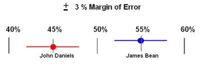
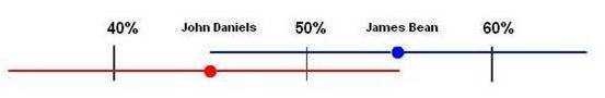
Now, If you've ever heard the news say a race is too close to call or there's a "statistical tie" it's because the width of both confidence intervals are overlapping enough that there's no clear leader. What does that mean? Imagine that a lot fewer people were surveyed for the poll taken by the Star-Tribune Newspaper and the margin of error was now +/- 6%. This new relationship is displayed in the figure below.
6% Margin of Error causes confidence intervals to overlap
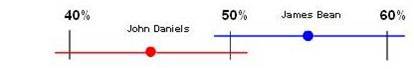
Notice how part of the confidence intervals overlap? The + 6% Margin of Error on the top of John Daniel's 45 % overlaps with the - 6% of Jim Bean's 55%. This means that if the poll were to be taken again, there's a reasonable chance that John Daniels might be leading over Jim Beam in the polls. So in this case, we can not be confident to say that James Bean is the leader.
In the above sections, we have discussed how confidence intervals come about and how they are influenced by sample size. Now if we are given a confidence interval, how should we interpret it?
For example, in a study of water samples randomly taken from a river polluted by crude oil, 95% CI of crude oil concentration is 20 to 60 ppm. This can be interpreted as "We are 95% confident that crude oil concentration is 40 ppm, with a margin of error of +/- 20 ppm".
Another example, in a study of effectiveness of the antidepressant buproprion for quitting smoking, we found 95% CI of proportion not smoking after six months of antidepressant buproprio treatment is 0.25 - 0.45 while 95% CI of proportion not smoking after six months of taking placebo (A placebo looks like the real drug but has no active ingredients, such as sugar pill) is 0.10 - 0.30. This can be interpreted as "We are 95% confident that the proportion not smoking after six months of antidepressant buproprio treatment is 0.35 ( (0.25 + 0.45)/2 = 0.35), with a margin of error +/-0.10 (0.35 +/-0.10 gives the range of 0.25 - 0.45)" and "We are 95% confident that the proportion not smoking after six months of taking placebo is 0.20 ( (0.10 + 0.30)/2 = 0.20), with a margin of error +/-0.10 (0.20 +/-0.10 gives the range of 0.10 - 0.30)".
Another example, in a study of breast cancer, we found 95% CI of RR of breast cancer for those women with high fat diet is 1.27 - 4.79. This can be interpreted as "We are 95% confident that the breast cancer risk of women who are on high fat diet is between 1.27 and 4.79 times as likely as those who are not on fat diet".
Imagine that you work for a city health department. Your city has had a chronic problem with E. coli outbreaks, particularly among children. You suspect one of the public pools (Oak Pool). If Oak Pool is causing the outbreak, you will need to close it.

You are trying to decide which of the following is closest to reality. Possible Realities:
After a recent outbreak, you surveyed people who swam at various public pools. You calculated the RR of E Coli illness for swimming at Oak Pool compared to other pools. Below are five alternative results. For which results would you act to close Oak Pool? For which would you eliminate Oak Pool as a suspected cause?
RR 95% CI____
Result 1 2.3 0.2 - 12.3
Result 2 2.3 0.6 - 7.1
Result 3 2.3 0.9 - 5.3
Result 4 2.3 1.3 - 3.9
Result 5 2.3 2.1 - 2.5
You can see that the RR in each case is the same, 2.3 - suggesting that the pool is the cause and you should close it. However, you recognize that there is uncertainty in estimating the true RR, and you want to avoid making a mistake in your decision to leave the pool open or to close it. In Result 5 (RR in the range of 2.1-2.5), the range of uncertainty is small and the entire range suggests that the pool is the cause. You could be confident in your decision to close it. At the other extreme, Result 1 (RR in the range of 0.2-12.3) has a very wide confidence interval. It includes the possibility that the pool increases your risk of disease, that it is unrelated to disease, and even that the pool protects you from disease. Clearly, you could not be much confident that a decision to close the pool would be a correct decision. You need more data.
Perhaps the toughest situation is Result 3. Here the confidence interval mostly suggests increased risk, but at the lower end it overlaps 1, suggesting that the pool has little or no effect on disease risk. Some researchers argue that if the confidence interval overlaps 1, you should conclude it has no effect - that is, the independent variable is NOT related to the dependent variable. However, this is not a wise approach for health professionals, since this simply increases the likelihood of having a false negative in order to avoid a false positive. Instead, you will have to use professional judgment. What is the potential cost of waiting for more information? What is the potential cost of acting, if you turn out to be wrong (a false positive)? Don't look for simple ways to make a decision in these cases; you must use your professional reasoning.
A final note on confidence intervals. Statisticians refer results 1 - 3 as "statistically not significant" since RRs overlap 1 suggesting it has no effect - that is the independent variables is NOT related to the dependent variables and results 4 - 5 "statistically significant" since RRs don't overlap 1 suggesting it has an effect. As we have pointed out earlier, statistical significance should NOT be the only factor in making professional decisions.
How likely is it that our sample (the descriptive statistic or measure of association observed in our sample) could have come from a population with characteristic, X, just by the luck of the draw? (X is a specific descriptive statistic or measure of association). For example, how likely is it that we could have gotten a sample with a relative risk of 2 by the "luck of the draw" from a population with relative risk of 1.0?
The basic question we are pursuing here is: How likely is it that this particular sample could come from this particular population? Occasionally, especially when we are dealing with descriptive statistics, we may know the value of the descriptive statistic for the population (such as mean height). Typically, however, we are dealing with measures of association and we have no idea what the value is for the population. This is why we usually begin with an assumption: that there is no connection between the two variables under study in the population and that the value for the measure of association reflects this (we commonly call this the "null hypothesis"). In other words, if we were studying the association between benzene exposure (exposed/unexposed) and leukemia (get it/don't get it) we would use relative risk (RR) as our measure of association. If there were no connection between benzene and leukemia the RR would equal 1. Thus RR=1 is our "null hypothesis" and we begin with the assumption that this is true for the population.
Say that we then observe a RR of 2 in the sample of subjects that we are studying. How likely is it that we could get a RR of 2 just by the "luck of the draw" if our population RR was 1? More precisely, how likely is it that, "just by the luck of the draw" we could get a RR that deviates at least this much from the null value of 1?
To answer our question, we use the appropriate Chance Assessment Tool (also known as "inferential statistic") to derive a p-value. In this case, since we are dealing with two dichotomous variables, the appropriate Chance Assessment Tool would be the Chi-square test. Let's assume that it identified a p-value of 0.06. This means that there is a 6% likelihood that we could get, by the "luck of the draw", a RR of 2 in our sample if the population from which the sample was drawn had a RR of 1. Another way of looking at it is that if we drew 100 samples (of the same sample size as the one we are studying) from a population with RR=1, only 6 of those samples would have an RR of 2 or more. A final way to interpret the p-values is that there is a 6% probability that chance could be responsible for the observed deviation from RR=1.
This suggests that it is relatively unlikely that we could have drawn our sample from a population with RR=1. In other words, our assessment of chance suggests that our original assumption about the population (our "null hypothesis") is wrong.
A final note on p-values. In the past, statisticians called p-values of 0.05 or less "statistically significant" and suggested that this meant you could reject your null hypothesis. The folly (and danger) in this mindless approach to decision-making should be apparent. The 0.05 level is strictly arbitrary. Why should a p-value of 0.055 force you to act as if there were no association between your variables? More importantly, rejecting your null hypothesis on the basis of a p-value alone makes sense only if you ignore the possible role of bias and confounding in explaining your results, which would be a foolish thing to do! Fortunately, researchers are slowly abandoning this myopic view of p-values.