Lesson Six
Measure of Association for Nominal and Ordinal Data - Finding Connections between Variables

Learning Objectives:

After successfully completing this lesson, students should be able to:

1. Choose appropriate measure of association for nominal and ordinal data

2. Calculate and interpret:

• Rates
• Rate Ratio or Relative Risk (RR)
• Attributable Risk (AR)
• Attributable Proportion (AP)

3. Generate measure of association for nominal and ordinal data using Epi Info.

Measures of Association (MOAs) for Nominal and Ordinal Data - Finding connections between variables

To find "causes" we look to our data for connections between an independent variable (potential causal factor) and a dependent variablele (outcome or problem). But how will we see this in our data? The answer is Measures of Association. That is, a measure of the association between the two variables.

It is important to note that all of the discussion that follows assumes we have eliminated alternative explanations for observed associations between variables, so we can be reasonably confident the associations are causal. This point will be covered in more detail later in the course.

When Both Variables Are Nominal - Compare proportions: Rates, Rate Ratio, Attributable Risk, Attributable Proportion

If we are concerned, for example, that exposure to benzene may cause leukemia, then we might do a study to see if refinery workers exposed to benzene have a greater risk of leukemia than those who are unexposed. 

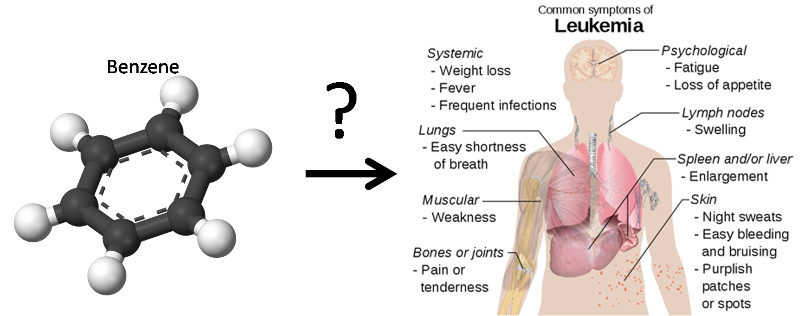
The following video might also help you to know more about acute myeloid leukemia (Note you can select full screen if you want).

But, how will the connection between leukemia and benzene exposure be evident in our data? Assume we collected the following data in our study:

Table 1. Leukemia rates and rate ratio (RR) for refinery workers by benzene exposure.

In our study, we noted the number of workers exposed to benzene and the number not exposed. We also noted how many workers in each group developed leukemia (note that both the dependent variable "Leukemia" and the independent variable "Benzene exposure" are nominal, i.e. Leukemia (Yes, or No) and Benzene exposure (Yes, or No). From this we can calculate the leukemia rate in each group:

[1]: 8.33 = (25/3,000) x 1,000;

[2]: 1.77 = (53/30,000) x 1,000

It is obvious, by comparing the leukemia rates in the two groups that the risk of leukemia is much higher among those exposed to benzene. We can better quantify this excess rate by taking a ratio of the two rates creating a rate ratio, or RR (also called a risk ratio, or the relative risk):

[3]: Risk ratio, or relative risk (RR)= 8.33/1.77 = 4.71

We interpret the rate ratio as follows:

 The risk of leukemia among exposed workers is 4.71 times as great as the risk among non-exposed workers.

This is very useful information. It suggests that benzene exposure dramatically increases one's risk of leukemia. Note here that non-exposed workers is used as the reference group. Reference group refers to the group in the denominator in calculating RR. In another word, when calculating RR, rate of reference group should always be the denominator. Once a group is used as a reference group, we don't need to calculate RR for that group (i.e. RR is not needed for a reference group).

Alternatively, we could subtract the rates instead of dividing them (Table 2). This is sometimes called Attributable Risk (AR), Risk Difference (RD), or Difference in Attack Rate (DAR).

Attributable Risk (AR), Risk Difference (RD), or Difference in Attack Rate (DAR)= 8.33 -1.77 = 6.56

Note there that non-exposed workers is again used as the reference group. In another word, when calculating AR or RD, rate of reference group should be the second term in subtraction.

Once a group is used as a reference group, we don't need to calculate AR or RD for that group (i.e. AR or RD is not needed for a reference group).

Table 2. Relative Risk (RR), Attributable Risk (AR) and Attributable Proportion (AP) for leukemia and benzene exposure among refinery workers.

Attributable Risk (AR) is a bit more difficult to interpret than RR but can be just as useful. In this case we could interpret Attributable Risk (AR) as follows:

In workers exposed to benzene, the amount of leukemia risk that is attributable (caused by) their exposure to benzene is 6.56/1000.

In other words, total leukemia risk among exposed workders is 8.33/1000, but only 6.56/1000 seems to be due to the benzene. The other 1.77/1000 seems to be due to other factors, since people have this risk of leukemia even when they are not exposed to benzene. Another way of saying this is that bezene exposure seems to increase ones risk of leukemia by 6.56/1000.

The Attributable Proportion (AP) states this in relative terms. By dividing the AR by the Leukemia Rate, we find the proportion of leukemia risk among exposed workers that seems to be due to benzene exposure. In this case, about 79% of exposed workders leukemia risk appears to be due to benzene exposure (6.56/8.33 x 100 = 79%). Or stated another way, if these workers had not been exposed to benzene, their luekimia risk would be about 79% less.

Have I Grasped the Key Concepts Here?

In a study of leukemia and benzene exposure among refinery workers, the following result is obtained (workers without benzene exposure is used as the reference group) :

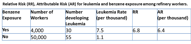
Based on the above table, answer the following questions.

Another Example on MOAs When Both Variables Are Nominal

You are the Director of a large urban county health department.  The rate of coronary heart disease (CHD) of your county is 2.1 times that of the state average. You know that both cigarette smoking and exposure to environmental tobacco smoke increase the risk of coronary heart disease.  You are considering proposing to the mayor a comprehensive smoking ban.  Comprehensive smoking bans prohibit smoking in workplaces, including public and private work sites, restaurants, and bars.  Studies have shown that comprehensive smoking bans reduce exposure to environmental tobacco smoke, whereas smoking restrictions, which permit designated smoking areas or provide separately ventilated sections, are not effective at preventing or eliminating exposure to environmental tobacco smoke.  Before you propose this idea to the mayor, you need more data to support it.  You came across an article entitled "The Impact of Massachusetts's Smoke-Free Workplace Laws on Acute Myocardial Infarction Deaths" in American Journal of Public Health, November 2010.  In this article, authors compared Acute Myocardial Infarction (AMI)^[1] mortality rate for Massachusetts residents aged 35 and older before and after implementation of the comprehensive state ban on smoking. 

The most important finding from this article is summarized in the table below:

[1] Myocardial infarction (MI) or acute myocardial infarction (AMI), commonly known as a heart attack. is the interruption of blood supply to a part of the heart, causing heart cells to die. This is most commonly due to occlusion (blockage) of a coronary artery following the rupture of a vulnerable atherosclerotic plaque, which is an unstable collection of lipids (fatty acids) and white blood cells (especially macrophages) in the wall of an artery.

[2]rate ratio is calculated using 'Before Ban" as the reference.

[3] 82.5/109.2 = 0.76 = 76%

[4] 18.1/22.2 = 0.82 = 82%

[5] 102.5/151.2 = 0.68 = 68%

[6] 432.2/567.1 = 0.76 = 76%

[7] 91.7/117.9 = 0.78 = 78%

[8] 74.5/101.7 = 0.73 = 73%

Now can you explain to the mayor and the public:

A. What does each of the rate ratio in the above table mean?

B. Was Massachusetts's Smoke-Free Workplace Laws effective in reducing AMI mortality rate across gender and age groups?

ANSWER:

In the above example, we are looking at the association between two nominal variables. One is smoking ban (Before, After) and the other is death from AMI (Yes, No). Similar to the benzene exposure and leukemia; instead of calculating leukemia rate among workers exposed to benzene and among workers not exposed to benzene, here, rate of death from AMI is calculated for before smoking ban and after smoking ban. In this article, not only the overall/total rates of AMI mortality (i.e. entire population was included) were compared before ban and after ban, rates of AMI mortality for subpopulation groups by either age or gender are also compared before ban and after ban.

A. Interpretation of each rate ratio in the table:

[3] 82.5/109.2 = 0.76 = 76%;

Overall, AMI mortality rate after ban is 0.76 times as great as the rate before the ban; or

Overall, AMI mortality rate after ban is 76% of the rate before the ban, or

Overall smoking ban reduce the AMI mortality rate by 24% (1 -76% = 24%).

[4] 18.1/22.2 = 0.82 = 82%;

For people aged 35-64, AMI mortality rate after ban is 0.82 times as great as the rate before the ban; or

For people aged 35-64, AMI mortality rate after ban is 82% of the rate before the ban; or

For people aged 35-64, smoking ban reduce the AMI mortality rate by 18% (1 -82% = 18%).

[5] 102.5/151.2 = 0.68 = 68%;

For people aged 65-74, AMI mortality rate after ban is 0.68 times as great as the rate before the ban; or

For people aged 65-74, AMI mortality rate after ban is 68% of the rate before the ban; or

For people aged 65-74, smoking ban reduce the AMI mortality rate by 32% (1 -68% = 32%).

[6] 432.2/567.1 = 0.76 = 76%;

For people aged 75 or older , AMI mortality rate after ban is 0.76 times as great as the rate before the ban;

For people aged 75 or older , AMI mortality rate after ban is 76% of the rate before the ban; or

For people aged 75 or older, smoking ban reduce the AMI mortality rate by 24% (1 -76% = 24%).

[7] 91.7/117.9 = 0.78 = 78%;

For males, AMI mortality rate after ban is 0.78 times as great as the rate before the ban; or

For males, AMI mortality rate after ban is 78% of the rate before the ban; or

For males, smoking ban reduce the AMI mortality rate by 22% (1 -78% = 22%).

[8] 74.5/101.7 = 0.73 = 73%;

For females, AMI mortality rate after ban is 0.73 times as great as the rate before the ban; or

For females, AMI mortality rate after ban is 73% of the rate before the ban; or

For females, smoking ban reduce the AMI mortality rate by 27% (1 -73% = 27%).

B. Was Massachusetts's Smoke-Free Workplace Laws effective in reducing AMI mortality rate across gender and age groups?

As we can see in rate ratios broken down by age groups and gender, all rate ratios shows a reduction (ratio ratios are less than 1) in AMI mortality rate after ban. So Massachusetts's Smoke-Free Workplace Laws effective was effective in reducing AMI mortality rate across gender and age groups.

Note the above example shows an application of MOAs in evaluating the effectiveness of certain intervention programs. In this case, intervention program reduced rate of certain disease, indicated by rate ratio of less than one.

One More Example on MOAs When Both Variables Are Nominal

You are an Environmental Health and Safety professional working with a plastic products producer. There are over 100 extrusion presses on the floor. The process begins by heating the stock material. It is then loaded into the container in the press. A dummy block is placed behind it where the ram then presses on the material to push it out of the die. Afterward the extrusion is stretched in order to straighten it. Frequently, when reaching into the press to remove the product, the worker sustains a burn to the forearm. 

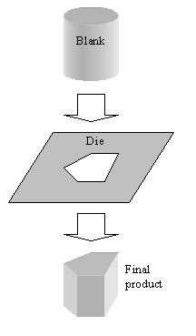
Above illustration shows extrusion of a round blank through a die.

You design a new guard to protect the worker against burns without interfering with the work process. To try your guard you select 10 test machines and install the guard. You also select 10 control machines without the new guard. You monitor the number of burns sustained by workers on each machine over the next two weeks. Your data are below. 

Number of burns sustained on 10 guarded and 10 un-guarded presses

MACH=press ID number, BURNS=number of burns in period, GUARD= presence of guard (1 - Yes, 0 - No)

A. Identify the subjects, dependent variable(s) and independent variable(s)

B. Construct a standard table and use the MOAs to determine the extent to which the guards seem to be working (does the presence of a guard reduce the risk of burns?). Explain your results using the MOAs. Clarity in your presentation (use a table) and your analysis of data are important. (NOTE: convert BURNS to a dichotomous variable, with 10 or more burns being "High")

ANSWER:

A. Subjects: Plastic extrusion presses

     Dependent Variable: Burns (Quantitative)

     Independent Variable: Presence of Guard (Nominal: Yes, or No)

B. In order to use RR as a measure of association, the BURN variable had to be converted from a quantitative variable to a dichotomous (categorical) variable. Burn counts of 10 or more were categorized as "High", below 10 was "Low". This produced the following results (Note the group with presence of guard is used as reference): 

[1] 20% = 2/10

[2] 60% = 6/10

[3] 3 = 60%/20%

Interpretation: the risk of high burn among machines without guard is 3 times as great as the risk among machines with the guard installed.

[4] 40% = 60% - 20%

Interpretation: Lack of guard seems to increase the risk of high burn by 40%

[5] 67% = 40%/60%

Interpretation: 67% of the high burn risk among machines without guard appears to be due to lack of the guard.

Comparing the 60% high burn rate among machines lacking the guard with the 20% burn rate among machine with the guard, the guard seems to be producing a dramatically lower burn rate. In fact machines without the guard are 3 times as likely to have a high burn rate as those with the guard installed. It strongly suggests that the guard should be installed of on all machines.

Have I Grasped the Key Concepts Here?

A study has been conducted to examine the impact of comprehensive smoking ban on AMI mortality rate and results are summarized in the table below (Note RR is calculated using before ban as the reference):

Based on above table, answer the following questions:

The following questions are based on this situation: You work with the City of Milwaukee Health Department. Recently, a large outbreak of Cryptosporidiosis has occurred, affecting tens of thousands of people. The following two videos describe some basic information on Cryptospordiosis and Cryptosporidium (Note you can select full screen if you want):

You suspect that the drinking water supply may be the cause.You randomly selected 30 residents and questioned them as to whether they have the symptoms of cryptosporidiosis and whether they drink the city water. Your results are summarized in the Table below.

Based on the table above, please answer the following questions (note, we will use group without city water consumption as the reference group in RR and AR calculation).

Practical Skills - How to Generate A Contingency Table, RR and AR using Epi Info?

The following video shows you how to generate a a contingency table (also referred to as cross tabulation or cross tab) that contains critical information needed for calculation of rate, RR and AR. Please note the procedure in this video also applies when independent variable is ordinal (discussed on pages 4-5 in this lesson). I have also included written instruction below for your reference.

Make sure you have told Epi Info to read the dataset you want to use before you can analyze it (If you forget how to do this, go to Lesson Two, Page 2 for a video on how to "Read a Dataset - 1^st Step of All"). After you have read the dataset in Epi Info,

• Go to "Statistics", select "Tables". Select an independent variable (i.e. possible causal factor) into the "Exposure Variable" window, and a dependent variable (i.e. a problem or an outcome) into the "Outcome Variable" window. In another word, the exposure variable is a variable that could influence or make a difference for the outcome variable. Let's say we want to examine if gender of a patient could influence or make a difference in someone's likelihood of infection, then we pick "GENDER" (i.e. causal factor/independent variable) into the "Exposure Variable" window and "INF" (i.e outcome/dependent variable) into the "Outcome Variable" window. Don't switch the two.
• Click "OK" and after a moment, a contingency table should appear in the output area under the title "TABLES GENDER INF". Scroll down and you should see RR and RD% (i.e. AR) under the title "Single Table Analysis". The following example will illustrate STEP BY STEP how to use Epi info to solve a particular problem using RR and RD% (i.e. AR) generated from Epi Info.

Using Epi Info to Solve a Problem

Let's go back to our Titanic dataset (remember you have used it in your homework assignment #2). As we investigate factors that may have influenced one's likelihood of survival in the accident, we may wonder whether "AGE" (nominal, adult vs. child) could be a factor associated with surviving in the accident. To find out, we need to use Epi Info to generate a contingency table, RR and AR using the "TABLES" command. Independent variable in this case is "AGE" (since it is a potentail causal factor) and dependent variable is "SURVIVED" (i.e. the outcome). The contingency table looks like below:

Note: AGE   (1 = adult, 0 = child); SURVIVED (1 = yes, 0 = no)

In addition, Epi Info also generated many statistics under the title "Single Table Analysis" as shown below

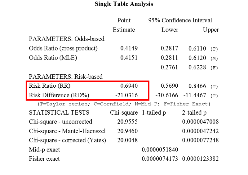
The two most important pieces of information relevant to us is the RR of 0.6940 and AR (i.e. RD% in the table) of -21% (Notice % is added since RD% is presented in the table). Now, naturally we wonder which (Adult or Child) is the reference when RR and AR is calculated by Epi Info. The answer is in the contingency table. The category listed in the top row (in this case, AGE = 0 (i.e. child) is used as the reference for RR and AR calculation. Now we can solve the problem!

RR of 0.6940 tells us that likelihood of surviving for an adults is only 0.694 times as great as the risk for a child.

AR of -21% tells us that being an adult seemed to decrease one's likelihood of surviving by 21%

So, age is a factor associated with one's likelihood of surviving.

If independent variable is an Ordinal Varilable (if independent variable is a nominal variable, see above for RR and AR)

Unfortunately Epi Info will not generate RR and RD% (i.e. AR) for each category of the ordinal variable, it will only generate a contingency table. So we will have to manually calculate RR and AR for each category of the ordinal variable. Now, how would we calculate RR and AR from a contingency table generated by Epi Info? Let's use the contingency table of "AGE" and "SURVIVED" from above as an example.

Note: AGE   (1 = adult, 0 = child); SURVIVED (1 = yes, 0 = no)

It is a very busy and confusing table. So, let's just focus on counts in the above table (ignore the % scores, just focus on the whole numbers) and rewrite the table into the following format:

Now, we can easily find out the survival rate for children and adults as well as RR and AR. We can choose any of the category as the reference category, let's use "Adult" as the reference here. Let's present them in a standard table with rates, RR and AR as below:

[1] 109 = 52+57

[2] 2092 = 1438 + 654

[3] 52% = 57/109

[4] 31% = 654/2092

[5] 1.7 = 52%/31%, the likelihood of survival for a child is 1.7 times as great as the likelihood for an adult.

[6] 21% = 52% - 31%, being a child seemed to increase the likelihood of survival by 21%.

When Independent Variable is Ordinal

When the independent variable is ordinal, use the same MOAs as you would if the independent variable were nominal - except look for a trend rather than simply a difference. For example, assume we were examining the relationship between childhood blood lead level and whether the child is diagnosed with a "learning disability", and we collected some data. However, before we dig into the data analysis, you might want to watch a couple of videos to understand some basic information on lead poisoning in childhood (Note you can select full screen if you want):

We get the following data (some columns were omitted to save space).

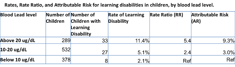
Table 3. Rates, Rate Ratio, and Attributable Risk for learning disabilities in children, by blood lead level.

Note the group of blood lead level below 10 ug/dL is used as the reference group.

[1] 16/127 = 0.126 = 12.6%

[2] 14/267 = 0.052 = 5.2%

[3] 4/183 = 0.022 = 2.2%

[4] 5.8 = 12.6%/2.2%;

Interpretation:  The risk of learning disability among children with blood lead level of above 20 ug/dl is 5.8 times as great as the risk among children with blood lead level below 10 ug/dl.

[5] 2.4 = 5.2%/2.2%;

Interpretation:The risk of learning disability among children with blood lead level of 10-20 ug/dl is 2.4 times as great as the risk among children with blood lead level below 10 ug/dl.

[6] 10.4% = 12.6%-2.2%;

Interpretation:  In children with blood level of above 20 ug/dl, the amount of learning disability risk that is attributable (caused by) their lead blood level is 10.5%; or Blood lead level of 20 ug/dl seems to increase a child's learning disability risk by 10.5%.

[7] 3.0%=5.2%-2.2%;

Interpretation: In children with blood level of 10-20 ug/dl, the amount of learning disability risk that is attributable (caused by) their lead blood level is 3.0%; or Blood lead level of 10-20 ug/dl seems to increase a child's learning disability risk by 3.0%.

[8] 82.5% = 10.4%/12.6%

Interpretation: 82.5% of learning disability risk in children with lead blood level of above 20 ug/dl appears to be due to their lead blood level; or if these children's lead blood level were reduced to below 10 ug/dl, their learning disability risk would be 82.5% less.

[9] 57.7% = 3.0%/5.2%

Interpretation: 57.7% of learning disability risk in children with lead blood level of 10-20 ug/dl appears to be due to their lead blood level; or if these children's lead blood level were reduced to below 10 ug/dl, their learning disability risk would be 57.7% less.

Note that we use the same MOAs we would if blood lead level had been nominal - rates, RR, and AR. However, because blood lead level is ordinal, we are looking primarily for a trend in these values. In this case, a trend is obvious. As blood lead level goes up, so does the rate of learning disabilities (and RR and AR and AP). This is strong evidence of a link between these two variables.

Have I Grasped the Key Concepts Here?

A study was conducted to examine the relationship between childhood lead blood level and whether a child has a learning disability or not. Results were summarized in the table below (Note the group of blood lead level below 10 ug/dL is used as the reference group here).

Based on the above table, answer the following questions:

Another Example of MOAs When Independent Variables Are Ordinal

You work in an urban health department in the tuberculosis treatment center, where patients with active TB come for monitored treatment. It is critical that patients return for treatment throughout the treatment period (several months), because stopping the treatment early can result in developing antibiotic resistance, making the disease much more difficult to treat. You are concerned that the distance the patient must travel is a major factor in determining whether they stay in the program.

You survey patients as they enter the program and then follow them to see if they complete the treatment. After 6 months, you have the following data: 

• Travel under 1 mile: Total patients: 117                Patients dropping out: 20
• Travel 1-3 miles: Total patients: 56                       Patients dropping out: 22
• Travel more than 3 miles: Total patients: 37         Patients dropping out: 27

A. Identify the subjects, dependent variable(s) and independent variable(s)

B. Construct a standard table and determine the extent to which the problem is related to the distance traveled. Explain your results, using the measures of association. Clarity in your presentation (use a table) and your analysis of data are important.

ANSWER

A. Subjects: Patients at TB treatment center

     Dependent Variable: Dropping out (Nominal: Yes, or No)

     Independent Variable: Travel distance (Quantitative)

B. The data can be summarized in a table such as the one below.

Note the group of traveling distance less than 1 mile is used as the reference group here.

[1] 17% = 20/117

[2] 39% = 22/56

[3] 73% = 27/37

[4] 2.3 = 39%/17%

Interpretation: The risk/likelihood of dropping out among patients who travel 1-3 miles is 2.3 times as great as the risk/likelihood among patients who travel under 1 mile.

[5] 4.3 = 73%/17%

Interpretation: The risk/likelihood of dropping out among patients who travel more than 3 miles is 4.3 times as great as the risk/likelihood among patients who travel under 1 mile.

[6] 22% = 39% - 17%

Interpretation: Traveling 1-3 miles seems to increase the risk/likelihood of dropping out by 22%

[7] 56% = 73% - 17%

Interpretation: Traveling more than 3 miles seems to increase the risk/likelihood of dropping out by 56%

Results indicate that the farther patients much come for treatment, the higher their drop out rate. Those who must travel 1-3 miles are more than twice as likely to drop out than those who travel less than a mile. Those who must travel over 3 miles are more than 4 times as likely to drop out as those who must travel less than a mile. Results suggest that locating treatment centers closer to patients, or perhaps providing them with transportation, could reduce the drop out rates dramatically.

One More Example of MOAs When Independent Variables Are Ordinal

You are a health educator working for American Cancer Society. One of the project you are involved is looking at "Interventions to increase colon cancer screening in Filipino Americans". According to CDC, colon cancer is the third leading cancer killer in the U.S.

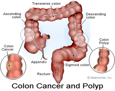
You may watch the video below to learn more on colon cancer screening (Note you can select full screen if you want to):

In this project, nearly 550 study participants were randomly assigned to one of three groups - two intervention groups and one control. Those in the intervention groups received an education session, printed take-home materials, a reminder letter, and a letter to physicians. The only difference between the two intervention groups was that one received a free take-home screening kit, while the other group did not. People in the control group had a session promoting physical activity. Six months after the intervention, participates are surveyed to see if they have completed the screening. The following data are collected:

• Intervention with free take-home screening kit: Total participants: 180               Participants completed screening: 54
• Intervention without free take-home screening kit: Total participants: 188            Participants completed screening: 45
• Control (i.e. no intervention): Total participants: 180          Participants completed screening: 16

A. Identify the subjects, dependent variable(s) and independent variable(s)

B. Construct a standard table and determine the extent to which the problem is related to the distance traveled. Explain your results, using the measures of association. Clarity in your presentation (use a table) and your analysis of data are important.

ANSWER

A. Subjects: Filipino Americans participated in the study

     Dependent Variable: Colon cancer screening (Nominal: Yes, or No)

     Independent Variable: Intervention (Ordinal: No; intervention w/o kit; intervention w kit)

B. The data can be summarized in a table such as the one below.

Note the control group is used as the reference group here.

[1] 54/180 = 30%

[2] 45/188 = 25%

[3] 16/180 = 89%

[4] 3.4 = 30%/8.9%; the likelihood of completing a colon screening test among participants who had gone through the intervention with free take-home screening kit is 3.4 times as great as the likelihood among participants who had not gone through any intervention.

[5] 2.8 =25%/8.9%; the likelihood of completing a colon screening test among participants who had gone through the intervention without free take-home screening kit is 2.8 times as great as the likelihood among participants who had not gone through any intervention.

Results indicate that the intervention particularly the intervention with free take-home screening kit are effective in getting people to complete a colon cancer screening test.

Note the above example shows another application of MOAs in evaluating effectiveness of certain intervention programs. In this case, the intervention increased rate of a good thing (i.e. colon screening test), indicated by rate ratios of greater than one.

Also notice, instead of saying "risk of a certain disease", here we used "the likelihood of a certain event" (i.e. the likelihood of completing colon screening test). Had we used the wording "the risk of completing a colon screening test", it would imply INCORRECTLY that colon screening test is a bad thing.

So in summary, if we want to talk about probability of a good thing happening, we typically say "the likelihood of a good thing is ....."; if we want to talk about probability of a bad thing happening, we typically say "the risk of a bad thing is ....".

Have I Grasped the Key Concepts Here?

A study was conducted to evaluate effectiveness of two intervention programs that aimed to increase colon cancer screening, results are summarized in the table below (Note the control group is used as reference group here):

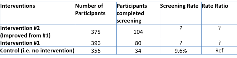
Based on above table, answer the following questions:

The following questions refer to this professional scenario:

You are a heath educator in a large county health department. You noticed that low birth weight (LBW) rate in your community is much higher than neighboring communities. You want to see if the cigarette consumption of mothers during pregnancy may have caused the low birth weight. You collected information on approximately 4000 pregnancies in terms of mothers cigarette consumption and whether a new born is considered low birth weight (LBW) or not. Results are summarized as the following (Note the nonsmoker is used as the reference group here):

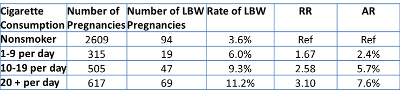
Based on the table above, answer the following questions: